ケプラーの第一法則#
(1609) The orbit of a planet is an ellipse with the Sun at one of the two foci.

楕円#
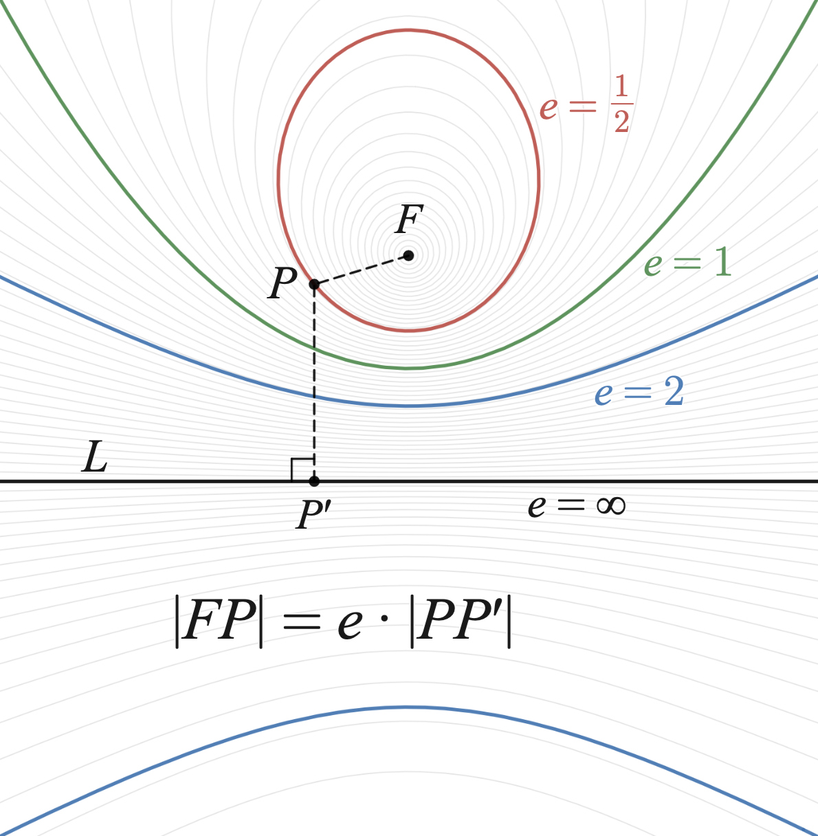
離心率 (eccentricity)#
-
Conic section - Wikipedia#Eccentricity,_focus_and_directrix
円錐曲線の離心率 \(e\) は、曲線上の点 \(P\) と焦点 \(F\) の距離と準線 \(L\) の距離の比である。
楕円は、準線を導入せずに定義できる。 楕円は、2つの焦点 \(F_{1}, F_{2}\) からの距離の和が等しい点 \(P\) の集合である。


楕円は、長軸の長半径 \(a\) と短軸の短半径 \(b\) を用いて二次方程式の解として定義できる。 $\( \frac{x^2}{a^2} + \frac{y^2}{b^2} = 1 \)$
この場合、離心率は次の式で表されるが、準線を用いて定義した離心率と等しい。
惑星の離心率#
!pip install -U lxml
Collecting lxml
  Using cached lxml-5.2.2-cp311-cp311-manylinux_2_28_x86_64.whl.metadata (3.4 kB)
Using cached lxml-5.2.2-cp311-cp311-manylinux_2_28_x86_64.whl (5.0 MB)
Installing collected packages: lxml
Successfully installed lxml-5.2.2
import pandas as pd
dfs = pd.read_html('https://en.wikipedia.org/wiki/Orbital_eccentricity')
dfs[1]
| Object | Eccentricity | |
|---|---|---|
| 0 | Triton | 0.00002 |
| 1 | Venus | 0.0068 |
| 2 | Neptune | 0.0086 |
| 3 | Earth | 0.0167 |
| 4 | Titan | 0.0288 |
| 5 | Uranus | 0.0472 |
| 6 | Jupiter | 0.0484 |
| 7 | Saturn | 0.0541 |
| 8 | Luna (Moon) | 0.0549 |
| 9 | Ceres | 0.0758 |
| 10 | Vesta | 0.0887 |
| 11 | Mars | 0.0934 |
| 12 | 10 Hygiea | 0.1146 |
| 13 | Makemake | 0.1559 |
| 14 | Haumea | 0.1887 |
| 15 | Mercury | 0.2056 |
| 16 | 2 Pallas | 0.2313 |
| 17 | Pluto | 0.2488 |
| 18 | 3 Juno | 0.2555 |
| 19 | 324 Bamberga | 0.3400 |
| 20 | Eris | 0.4407 |
| 21 | Nereid | 0.7507 |
| 22 | Sedna | 0.8549 |
| 23 | Halley's Comet | 0.9671 |
| 24 | Comet Hale-Bopp | 0.9951 |
| 25 | Comet Ikeya-Seki | 0.9999 |
| 26 | Comet McNaught | 1.0002[a] |
| 27 | C/1980 E1 | 1.057 |
| 28 | ʻOumuamua | 1.20[b] |
| 29 | 2I/Borisov | 3.5[c] |
# 火星の離心率
float(dfs[1][dfs[1]['Object'] == 'Mars'].iloc[0]['Eccentricity'])
0.0934
# 地球の離心率
float(dfs[1][dfs[1]['Object'] == 'Earth'].iloc[0]['Eccentricity'])
0.0167
dfs = pd.read_html('https://en.wikipedia.org/wiki/Mars')
dfs[0]
| 0 | 1 | 2 | 3 | |
|---|---|---|---|---|
| 0 | Mars in true color,[a] as captured by the Hope... | Mars in true color,[a] as captured by the Hope... | NaN | NaN |
| 1 | Designations | Designations | NaN | NaN |
| 2 | Adjectives | Martian | NaN | NaN |
| 3 | Symbol | NaN | NaN | NaN |
| 4 | Orbital characteristics[1] | Orbital characteristics[1] | NaN | NaN |
| 5 | Epoch J2000 | Epoch J2000 | NaN | NaN |
| 6 | Aphelion | 249261000 km (1.66621 AU)[2] | NaN | NaN |
| 7 | Perihelion | 206650000 km (1.3814 AU)[2] | NaN | NaN |
| 8 | Semi-major axis | 227939366 km (1.52368055 AU)[3] | NaN | NaN |
| 9 | Eccentricity | 0.0934[2] | NaN | NaN |
| 10 | Orbital period (sidereal) | 686.980 d (1.88085 yr; 668.5991 sols)[2] | NaN | NaN |
| 11 | Orbital period (synodic) | 779.94 d (2.1354 yr)[3] | NaN | NaN |
| 12 | Average orbital speed | 24.07 km/s[2] | NaN | NaN |
| 13 | Mean anomaly | 19.412°[2] | NaN | NaN |
| 14 | Inclination | 1.850° to ecliptic5.65° to Sun's equator1.63° ... | NaN | NaN |
| 15 | Longitude of ascending node | 49.57854°[2] | NaN | NaN |
| 16 | Time of perihelion | 2022-Jun-21[5] | NaN | NaN |
| 17 | Argument of perihelion | 286.5°[3] | NaN | NaN |
| 18 | Satellites | 2 (Phobos and Deimos) | NaN | NaN |
| 19 | Physical characteristics | Physical characteristics | NaN | NaN |
| 20 | Mean radius | 3389.5 ± 0.2 km[b] [6] (2106.1 ± 0.1 mi) | NaN | NaN |
| 21 | Equatorial radius | 3396.2 ± 0.1 km[b] [6] (2110.3 ± 0.1 mi; 0.533... | NaN | NaN |
| 22 | Polar radius | 3376.2 ± 0.1 km[b] [6] (2097.9 ± 0.1 mi; 0.531... | NaN | NaN |
| 23 | Flattening | 0.00589±0.00015[5][6] | NaN | NaN |
| 24 | Surface area | 1.4437×10⁸ km2[7] (0.284 Earths) | NaN | NaN |
| 25 | Volume | 1.63118×10¹¹ km3[8] (0.151 Earths) | NaN | NaN |
| 26 | Mass | 6.4171×10²³ kg[9] (0.107 Earths) | NaN | NaN |
| 27 | Mean density | 3.9335 g/cm3[8] | NaN | NaN |
| 28 | Surface gravity | 3.72076 m/s2 (0.3794 g0)[10] | NaN | NaN |
| 29 | Moment of inertia factor | 0.3644±0.0005[9] | NaN | NaN |
| 30 | Escape velocity | 5.027 km/s (18100 km/h)[11] | NaN | NaN |
| 31 | Synodic rotation period | 1.02749125 d[12] 24h 39m 36s | NaN | NaN |
| 32 | Sidereal rotation period | 1.025957 d 24h 37m 22.7s[8] | NaN | NaN |
| 33 | Equatorial rotation velocity | 241 m/s (870 km/h)[2] | NaN | NaN |
| 34 | Axial tilt | 25.19° to its orbital plane[2] | NaN | NaN |
| 35 | North pole right ascension | 317.68143°[6] 21h 10m 44s | NaN | NaN |
| 36 | North pole declination | 52.88650°[6] | NaN | NaN |
| 37 | Albedo | 0.170 geometric[13]0.25 Bond[2] | NaN | NaN |
| 38 | Temperature | 209 K (−64 °C) (blackbody temperature)[14] | NaN | NaN |
| 39 | Surface temp. min mean max Celsius −110 °C[15]... | Surface temp. min mean max Celsius −110 °C[15]... | NaN | NaN |
| 40 | Surface temp. | min | mean | max |
| 41 | Celsius | −110 °C[15] | −60 °C[16] | 35 °C[15] |
| 42 | Fahrenheit | −166 °F[15] | −80 °F[16] | 95 °F[15] |
| 43 | Surface absorbed dose rate | 8.8 μGy/h[17] | NaN | NaN |
| 44 | Surface equivalent dose rate | 27 μSv/h[17] | NaN | NaN |
| 45 | Apparent magnitude | −2.94 to +1.86[18] | NaN | NaN |
| 46 | Absolute magnitude (H) | −1.5[19] | NaN | NaN |
| 47 | Angular diameter | 3.5–25.1″[2] | NaN | NaN |
| 48 | Atmosphere[2][20] | Atmosphere[2][20] | NaN | NaN |
| 49 | Surface pressure | 0.636 (0.4–0.87) kPa 0.00628 atm | NaN | NaN |
| 50 | Composition by volume | 95.97% carbon dioxide 1.93% argon 1.89% nitrog... | NaN | NaN |
| 51 | NaN | NaN | NaN | NaN |
dfs[0][dfs[0][0] == 'Eccentricity']
| 0 | 1 | 2 | 3 | |
|---|---|---|---|---|
| 9 | Eccentricity | 0.0934[2] | NaN | NaN |
近日点、遠日点#
Apsis - Wikipedia (近点・遠点)
Apsis - Wikipedia#Perihelion_and_aphelion (近日点・遠日点)

火星の次の近日点・遠日点通過日#
!pip install -U astronomy-engine
Requirement already satisfied: astronomy-engine in /opt/conda/lib/python3.11/site-packages (2.1.19)
import astronomy
a0 = astronomy.SearchPlanetApsis(astronomy.Body.Mars, astronomy.Time.Now())
a0
Apsis(Time('2025-04-16T22:54:51.374Z'), ApsisKind.Apocenter, dist_au=1.6660577981008962)
a1 = astronomy.NextPlanetApsis(astronomy.Body.Mars, a0)
a1
Apsis(Time('2026-03-26T07:06:54.273Z'), ApsisKind.Pericenter, dist_au=1.3812758063827724)
# 火星の離心率
abs(a0.dist_au - a1.dist_au) / (a0.dist_au + a1.dist_au)
0.09345284392201504
%%ai_ask
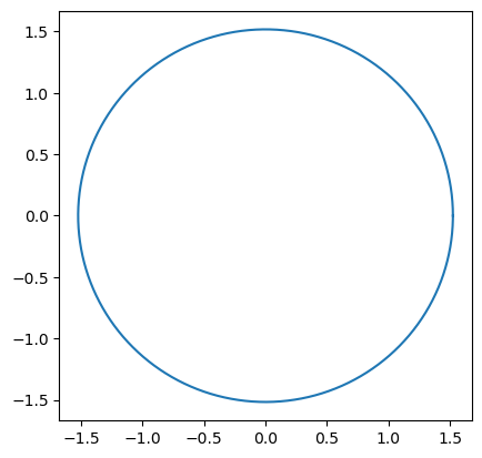
jupyterのpythonで火星の公転軌道と同じ離心率の楕円を描く
以下のコードを実行することで、jupyterのpythonで火星の公転軌道と同じ離心率の楕円を描くことができます。
import matplotlib.pyplot as plt
import numpy as np

a = 1.524 # 火星の軌道長半径
e = 0.0934 # 火星の離心率

b = a * np.sqrt(1 - e**2) # 火星の軌道短半径

theta = np.linspace(0, 2*np.pi, 1000) # 角度を0から2πまで1000分割

x = a * np.cos(theta) # x座標
y = b * np.sin(theta) # y座標

plt.plot(x, y) # 楕円を描画
plt.gca().set_aspect('equal', adjustable='box') # アスペクト比を調整
plt.show() # 描画
このコードでは、matplotlibとnumpyを使用しています。また、火星の軌道長半径と離心率を変数に代入し、楕円のx座標とy座標を計算しています。最後に、plot関数で楕円を描画し、set_aspect関数でアスペクト比を調整しています。
import matplotlib.pyplot as plt
import numpy as np

a = 1.524 # 火星の軌道長半径
e = 0.0934 # 火星の離心率

b = a * np.sqrt(1 - e**2) # 火星の軌道短半径

theta = np.linspace(0, 2*np.pi, 1000) # 角度を0から2πまで1000分割

x = a * np.cos(theta) # x座標
y = b * np.sin(theta) # y座標

plt.plot(x, y) # 楕円を描画
plt.gca().set_aspect('equal', adjustable='box') # アスペクト比を調整
plt.show() # 描画
%%ai_ask
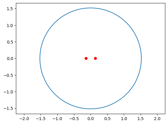
jupyterのpythonで火星の公転軌道と同じ離心率の楕円を描く。
その際に、2つの焦点を同時に描く。
以下のコードを使用して、Jupyter Notebook上で火星の公転軌道と同じ離心率の楕円を描くことができます。また、楕円の2つの焦点も同時に描かれます。
import matplotlib.pyplot as plt
import numpy as np

a = 1.524 # 長軸半径
e = 0.0934 # 離心率

b = a * np.sqrt(1 - e**2) # 短軸半径
c = e * a # 焦点間の距離

# 楕円の描画
theta = np.linspace(0, 2*np.pi, 1000)
x = a * np.cos(theta)
y = b * np.sin(theta)
plt.plot(x, y)

# 焦点の描画
plt.plot([-c, c], [0, 0], 'ro')

plt.axis('equal')
plt.show()
このコードでは、aとeをそれぞれ長軸半径と離心率に設定し、短軸半径と焦点間の距離を計算しています。そして、np.linspace()を使用して楕円の描画に必要な角度を生成し、np.cos()とnp.sin()を使用して楕円の座標を計算しています。最後に、plt.plot()を使用して楕円と焦点を描画し、plt.axis('equal')を使用してアスペクト比を調整しています。
import matplotlib.pyplot as plt
import numpy as np

a = 1.524 # 長軸半径
e = 0.0934 # 離心率

b = a * np.sqrt(1 - e**2) # 短軸半径
c = e * a # 焦点間の距離

# 楕円の描画
theta = np.linspace(0, 2*np.pi, 1000)
x = a * np.cos(theta)
y = b * np.sin(theta)
plt.plot(x, y)

# 焦点の描画
plt.plot([-c, c], [0, 0], 'ro')

plt.axis('equal')
plt.show()
地球の次の近日点・遠日点通過日#
a0 = astronomy.SearchPlanetApsis(astronomy.Body.Earth, astronomy.Time.Now())
a0
Apsis(Time('2025-01-04T13:22:32.083Z'), ApsisKind.Pericenter, dist_au=0.9833286160393861)
a1 = astronomy.NextPlanetApsis(astronomy.Body.Earth, a0)
a1
Apsis(Time('2025-07-03T20:11:47.601Z'), ApsisKind.Apocenter, dist_au=1.0166463687470069)
# 地球の離心率
abs(a0.dist_au - a1.dist_au) / (a0.dist_au + a1.dist_au)
0.01665908471909173
%%ai_continue
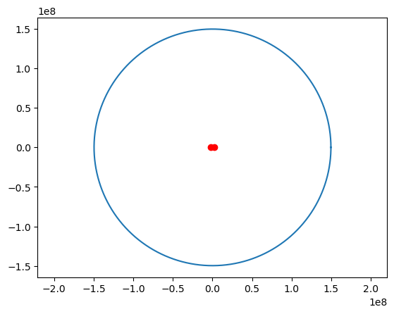
jupyterのpythonで地球の公転軌道と同じ離心率の楕円を描く。
その際に、2つの焦点を同時に描く。
以下のコードを使用して、Jupyter Notebook上で地球の公転軌道と同じ離心率の楕円を描くことができます。また、楕円の2つの焦点も同時に描かれます。
import matplotlib.pyplot as plt
import numpy as np

a = 1.496e8 # 長軸半径(単位:km)
e = 0.0167 # 離心率

b = a * np.sqrt(1 - e**2) # 短軸半径
c = e * a # 焦点間の距離

# 楕円の描画
theta = np.linspace(0, 2*np.pi, 1000)
x = a * np.cos(theta)
y = b * np.sin(theta)
plt.plot(x, y)

# 焦点の描画
plt.plot([-c, c], [0, 0], 'ro')

plt.axis('equal')
plt.show()
このコードでは、aとeをそれぞれ長軸半径と離心率に設定し、短軸半径と焦点間の距離を計算しています。そして、np.linspace()を使用して楕円の描画に必要な角度を生成し、np.cos()とnp.sin()を使用して楕円の座標を計算しています。最後に、plt.plot()を使用して楕円と焦点を描画し、plt.axis('equal')を使用してアスペクト比を調整しています。
なお、地球の公転軌道の長軸半径は約1.496×10^8 km、離心率は約0.0167です。
import matplotlib.pyplot as plt
import numpy as np

a = 1.496e8 # 長軸半径(単位:km)
e = 0.0167 # 離心率

b = a * np.sqrt(1 - e**2) # 短軸半径
c = e * a # 焦点間の距離

# 楕円の描画
theta = np.linspace(0, 2*np.pi, 1000)
x = a * np.cos(theta)
y = b * np.sin(theta)
plt.plot(x, y)

# 焦点の描画
plt.plot([-c, c], [0, 0], 'ro')

plt.axis('equal')
plt.show()
まとめ#
import numpy as np
import matplotlib.pyplot as plt
import matplotlib.collections as mc
import matplotlib.patches as mp
theta = np.linspace(0, 2*np.pi, 100)
#epsilon = 0.6
#epsilon = 0.9673 # 1P/Halley
#epsilon = 0.0934 # mars
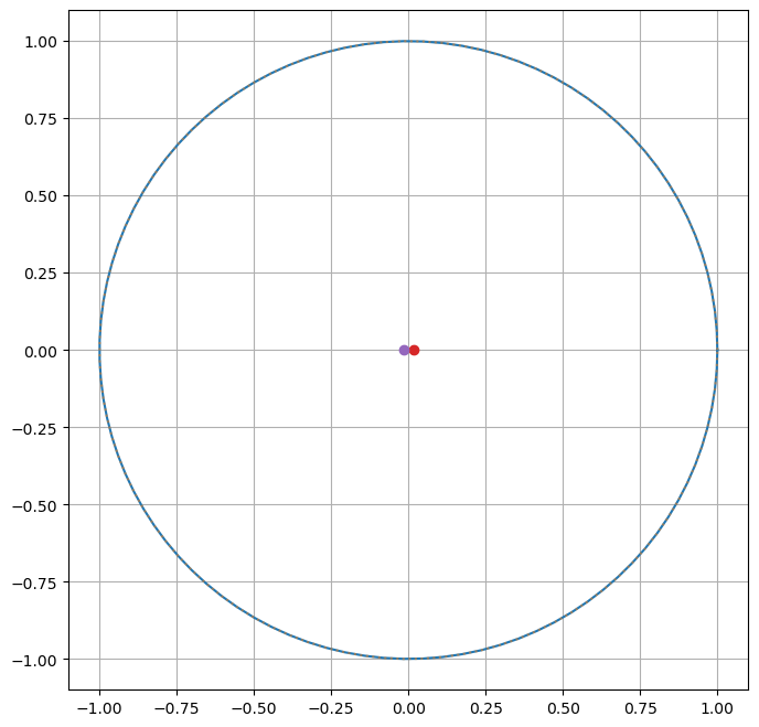
epsilon = 0.0167 # earth
a=1
b= np.sqrt(a**2-epsilon**2)
print(a, b, a*epsilon)
1 0.99986054527619 0.0167
ax = plt.figure(figsize=(16,8)).add_subplot()
ax.set_aspect('equal')

X0 = np.cos(theta)
Y0 = b * np.sin(theta)
ax.plot(X0,Y0)

X1 = np.cos(theta)
Y1 = np.sin(theta)
ax.plot(X1,Y1, ':', alpha=.5)

l = mc.LineCollection([[(a/epsilon,-1),(a/epsilon,1)]])
#ax.add_collection(l)

ax.plot(0,0,'x')
ax.plot( a*epsilon, 0, 'o')
ax.plot(-a*epsilon, 0, 'o')

plt.grid()
plt.show()